Introduction to Forecasting
Forecasting is a crucial process for several industries and is an essential process for financial institutions.
All procedures that over the years have been developed to address the problem of forecasting have several elements in common:
- Time
- Underlying uncertainty
- Eventually, these procedures are always wrong
- Always have a purpose or objective
There are several approaches to forecasting:
The time-series approach is the one taken by us and is essentially based on the idea that history repeats itself, at least approximately. It is generally based on the numerical series of the quantity you’re trying to predict.
The causal approach assumes that there is a reason behind the patterns you’re seeing. You must understand the reason and use that knowledge to generate the forecast.
The judgmental approach is simple, it assumes that someone else knows and can tell you the right answer. You essentially have to gather the knowledge and opinions of other people who are in a position to know what the demand will be, what the price will be, what the whatever quantity we’re predicting will be.
The experimental approach is useful when we’re dealing with new items and we have no other information upon which to base a forecast. You conduct an experiment on a small group of customers and then extrapolate the results to a larger group.
Although all approaches have been used in the past for the purpose of forecasting, the time series approach is the one most widely used for forecasting, partially because it is “anonymous” i.e. not biased by the judgment required in judgmental, causal and experimental approaches, partially because it is based on no assumptions (right or wrong) on the world you’re trying to model and partially because they are easy to use with modern computers.
Time-series Forecasting
A time-series is a set of quantities related to a process taken at regular intervals. For example the water outbound flow from a lake, the price of a stock, the lung cancer mortality are classical time series examples.
The time series forecasting procedures implemented in our tool are useful for logistic series (like the demand for a specific item or service), for financial series (like the price of the Microsoft share), Nature series (like the temperature measured in Central Park) and health related time series (like the lung cancer mortality).
We intend our forecasts to be very accurate but we do not expect them to be error free so time series forecasting must be applied and gives better results when:
- We intend to produce short term forecasts.
- The time series has ‘good’ statistical properties (it is not too short and it is not too variable).
We will use the following notation:
- Xt to represent the observed quantity at time t.
- X’t to represent the forecast at time t.
- et = Xt – X’t to measure the forecast error at time t.
In time series forecasting we assume that the data consists of data patterns that are the subject matter of our interest and noise that is uninteresting and random or simply cannot be forecasted.
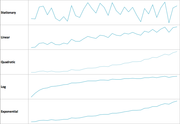
Typical patterns we will analyze are the trend, the seasonality and the cycle.
Types of Trend
The trend is the consistent behavior of the series to move in a specified direction, towards new highs or towards new lows.
Seasonality and Cycles
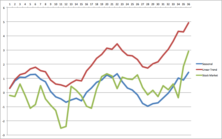
Seasonality is the consistent behavior of the series to move through high and low periods that are directly related to the time (and more specifically to the time of the year, for example in summer you sell more air conditioning than in winter and this is consistently true in the north of the world every year). The cycle is a periodic movement not related to the calendar.


